TechTool
» Statics 23
» Statics 22
» Statics 21
» Statics 20
» Statics 19
» Statics 18
» Statics 17
» Statics 16
» Statics 15
» Statics 14
» Statics 13
» Statics 12
» Statics 11
» Statics 10
» Statics 9
» Statics 8
» Statics 7
» Statics 6
» Statics 5
» Statics 4
» Statics 3
» Statics 2
» Statics 1

The World of Statistics – 1,2
By Dr. Magdi Abadir, PhD
Article – 7: The Central Tendency (3)
4. The median of grouped data
The last article discussed the determination of the median of ungrouped data. In the present article, the method used to obtain the median value of grouped data will be discussed.In many cases, one may be faced with a set of grouped data which are best represented by their median value. A typical example which is commonly encountered when dealing with particulate solids deserves detailed explanation.
In the building industry, chemical industry as well as in ore dressing and several other practical applications, one deals with “particulate solids”. This is a substance composed of more or less small particles of different size, such as sand, cement, crushed stone, pebbles, fine powders etc. These can be sorted to different size fractions by several methods, the easiest one being by sieving over a set of screens with different openings arranged from the biggest to the finest opening from top to bottom (Figure 1). A pan is located below the finest screen to collect fine dust.
The mass retained between each two consecutive sieves is determined and the openings of the two sieves noted. The first two rows in the following table represent a typical “Particle size distribution” of a sample of sand.
The total mass is obtained by summing up the individual masses (row 2). It equals 383.72 g. The percentage of sand having a certain size range is obtained by dividing the mass over that range by the total mass and multiplying by 100. For example, the percent sand (by mass) in the 0.590 – 0.834 size range (Sixth column) = 100× = 7.7%. The third row of the table has been set up this way. The total sum of the percentages of the third row = 100%.
One last set of calculations consist of obtaining the “cumulative distribution”, that is, the percentage of sand particles (by mass) with a size lower than a specific size. This is obtained by first adding a fourth row in which the smallest size in each size interval is placed, the pan being assumed to be of size = 0 mm. Finally, the fifth row is obtained by adding up the percent mass fractions in the third row in a cumulative way: for example, the mass percent of sand having a size less than 0.295 mm (Column 4) = 0.23 + 5.92 + 23.04 + 26.66 = 55.85%. The “cumulative plot” is carried out by plotting the percentages in row (5) against the particle sizes in row (4). (Figure 2)
| Size interval mm | pan– 0.074 | 0.074 – 0.147 | 0.147 – 0.295 | 0.295 – 0.417 | 0.417 – 0.590 | 0.590 – 0.834 | 0.834 – 1.180 | 1.180 – 1.668 |
| Mass g | 0.89 | 22.7 | 88.4 | 102.3 | 125.6 | 29.55 | 14.28 | 0 |
| % By mass | 0.23 | 5.92 | 23.04 | 26.66 | 32.73 | 7.7 | 3.72 | 0 |
| Size mm | 0 | 0.074 | 0.147 | 0.295 | 0.417 | 0.590 | 0.834 | 1.180 |
| % with size < than | 0.23 | 6.15 | 29.19 | 55.85 | 88.58 | 96.28 | 100 | 100 |
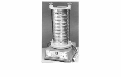
Fig (1): Set of sieves [1]
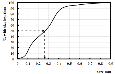
Fig (2): Determination of the median of a distribution
The particle size corresponding to 50% cumulative mass percent is the median of the distribution and is usually determined to be the most suitable average to represent the fineness in a particle size distribution. It is usually quoted as D50. In Figure (2), D50 ≈ 0.26 mm.
Reference:
Malewski J. “On accuracy of sieve analyses” Proc. Annual Conf. Aggregates, KruszMin’ 17. Kudova Zdrój – Wroclaw, Poland (2017) Vol (1): 103 – 111
N.A. Weiss “Elementary Statistics” Pub. Pearson, 9th Ed. (2016), Chapter 3(1)
| Dr. Magdi Fouad Abadir, Ph. D.: Dr. M. F. Abadir is currently a professor with the Chemical Engineering Department at the Faculty of Engineering, University of Cairo, Egypt. His major interests are in the fields of high temperature science and technology. During his career, he has supervised more than 110 MSc and PhD theses and published more than a hundred papers mostly in international peer review journals. He currently teaches courses in High Temperature Technology and Industrial Statistics. He is also a consultant for several industrial businesses. |


