TechTool
» Statics 23
» Statics 22
» Statics 21
» Statics 20
» Statics 19
» Statics 18
» Statics 17
» Statics 16
» Statics 15
» Statics 14
» Statics 13
» Statics 12
» Statics 11
» Statics 10
» Statics 9
» Statics 8
» Statics 7
» Statics 6
» Statics 5
» Statics 4
» Statics 3
» Statics 2
» Statics 1

The World of Statistics (1)
By Dr. Magdi Abadir, PhD
Article – 13: Measures of Dispersion (3)
2.3 The standard deviation and coefficient of variation of ungrouped data
Suppose a housewife intends to revamp her kitchen, seeking a reasonable price with acceptable quality. To that aim, she makes a search and limits her choices to seven offers forming the following set ($):S={48000 ,62000 ,65000 ,37000,42000,60000,46000}
Meanwhile, her husband is renewing his car and makes a short list of his preferences, the prices of which form the following set:
S'={28000 ,42000 ,55000 ,37000,45000,27000}
The average price of a kitchen is about $51,430 and the range of prices = 65,000 – 37,000 = $28,000. On the other hand, the average price of a car is about $37,500 and the range of prices = 55,000 – 27,000 = $28,000
We notice that both kitchen and car possess the same price range. This means that their ranges cannot decide about which of the two price lists is more scattered. Obviously, the limited amount of data in each case prevents applying the percentile measure for dispersion.
We introduce a third measure of dispersion, known as the standard deviation, with the following curious definition:
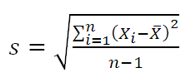
In that equation, X_i stands for the different values of the variable (here the price in USD) while X ̅ is the mean (average) value of these prices. The symbol
 stands for the sum
  Standard deviation has the same units as the original variable (Here it is $). A high standard deviation means a more dispersed distribution.
 Calculations for the standard deviation of both kitchen and car prices are summarized in the table.
| X | 48000 | 62000 | 65000 | 37000 | 42000 | 60000 | 46000 |
| X-X ̅ | -3429 | 10571 | 13571 | -14429 | -9429 | 8571 | -5429 |
| (X-X ̅ )^2 | 11755102 | 111755102 | 184183673 | 208183673 | 88897959 | 73469388 | 29469388 |
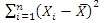
The sum of the third row
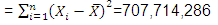
This sum is then divided by (n-1)=(7-1)=6 to obtain 117,952,381. The standard deviation for kitchen prices is then calculated by taking the square root of that number. One obtains:
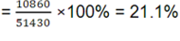
s (kitchen prices)=$10860
If similar calculations are carried out for car prices, it will yield:
Average price X ̅ = $37,500
s (car prices)=$10,596
The two standard deviations seem too close to judge about their relative dispersions. However, a necessary condition for proper comparison is that the two distributions should have equal average values. This is not the case in the present situation as the average price of kitchens = $51,430 while it is about $37,500 for cars. To take into consideration the difference between the two averages, we introduce one last measure for dispersion, which is the Coefficient of Variation (CV) defined by:

For kitchens: CV
For cars: CV
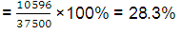
The higher CV for car prices indicates that their prices are more scattered than those of kitchens.
References:
(1) A.G. Bluman “Elementary Statistics” 8th edition. Mc Graw-Hill, 2012, Chapter 3,
| Dr. Magdi Fouad Abadir, Ph. D.: Dr. M. F. Abadir is currently a professor with the Chemical Engineering Department at the Faculty of Engineering, University of Cairo, Egypt. His major interests are in the fields of high temperature science and technology. During his career, he has supervised more than 110 MSc and PhD theses and published more than a hundred papers mostly in international peer review journals. He currently teaches courses in High Temperature Technology and Industrial Statistics. He is also a consultant for several industrial businesses. |


