Manageria
» Jan 2026
» July 2025
» Jan 2025
» July 2024
» Jan 2024
» July 2023
» Jan 2023
» Oct 2022
» July 2022
» Apr 2022
» Jan 2022
» Oct 2021
» July 2021
» Apr 2021
» Jan 2021


Add To What You Know
Prepared by: "Optimanage.com"
Determining the Economic Order Quantity (EOQ)(1)
The technique of determining the EOQ helps businesses to find:When to order new materials for inventory.
How much to order to be cost effective.
It is important to know that there are costs for keeping inventory. These costs are mainly:
Carrying Costs: Storing, Insurance, Spoilage, Theft, etc.
Ordering Costs: Clerical Labor, Forms, Order Processing Labor, etc.
Note that Carrying Costs and Ordering Costs are in directly related. That is to say that one of these cost goes up (increase), the other cost goes down (decrease).
The total Inventory Costs are equal to Carrying Costs plus Ordering Costs:
Total Inventory Costs = Carrying Costs + Ordering Costs
Inventory CT = Cc + Oc (1)
The order quantity with the lowest costs is called the “Economic Order Quantity – EOQ”. See Figure – 1.
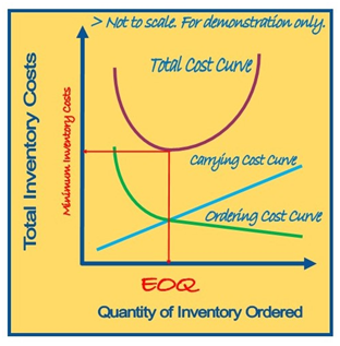
Figure – 1
Inventory Costs
Now consider a Company K; it is using 5 units of inventory every week (5 units/week). Note the following:
Inventory usage is constant.
Maximum inventory is on the first day.
Lowest inventory is on the last day.
Weekly use of inventory is 5 units to translate to 1 unit/day.
Total annual demand will be: 5 units/week X 52 weeks = 260 units.
There will be 52 orders/year; each order will be for 5 units.
At this point we are not sure if 5 units are the most economic order size. Nonetheless, we can determine the most economic order size because we know that at that point, which is EOQ, Carrying costs are equal to the Ordering costs. The EOQ is also known as Q*. See Figure – 2.
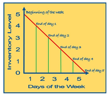
Figure – 2
Pattern of Inventory Usage
To find EOQ we will need the following elements:
Q = number of units ordered
Q* = optimal amount of each inventory order
D = annual demand of units of inventory
Oc = cost per each inventory order
Cc = cost of carrying each unit of inventory for a year
To find EOQ (Q*):
Find ordering costs:
| Ordering costs | = (number of orders/year) X (cost/order) |
| = annual demand of units/number of units per order X cost/order | |
| = (D / Q) (Oc) |
| Ordering costs | = (number of orders/year) X (cost/order) |
| = annual demand of units/number of units per order X cost/order | |
| = (D / Q) (Oc) |
Find average inventory level:
Average inventory level = (order quantity/2) (carrying cost/unit per year)
Carrying costs = (Q/2) Cc
To find Q*, the ordering costs are set equal to carrying costs.
(D / Q) Oc = (Q / 2) Cc
| Reversing terms: | Q2 Cc = 2 D Oc |
| solving for Q2: | Q2 = (2 D Oc) / Cc |
| solve for Q: | Q = √ (2 D Oc) / Cc |
| Reversing terms: | Q2 Cc = 2 D Oc |
| solving for Q2: | Q2 = (2 D Oc) / Cc |
| solve for Q: | Q = √ (2 D Oc) / Cc |
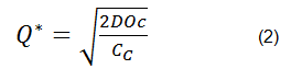
Since Cc were set to equal Oc. Then Q = Q* = EOQ Therefore:
Look at the following example:
A company has a demand of 25000 units of a material
Cost of order for each unit is $10
Carrying cost per year is $2 / unit
What is the Q* for the company to minimize inventory costs?
Using equation (2) to find Q*:
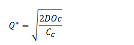
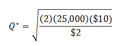
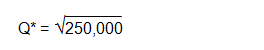
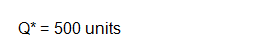
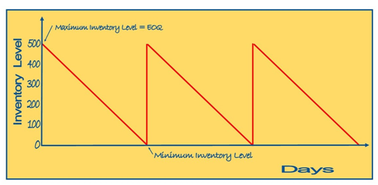
Figure – 3
Pattern of inventory usage for EOQ=500 units
From the above and since demand is 25,000 units, there will be 50 orders per year (see Figure – 3).
| Number of orders per year | = 25,000 units/ 500 units per order |
| = 50 orders per year |
| Number of orders per year | = 25,000 units/ 500 units per order |
| = 50 orders per year |
The above discussion and example represent the simplest of cases for determining EOQ. Any change in the operating conditions of inventory for a company or business will need to recalculate EOQ or Q* for the new case.
References:
(1) Patrick J. Montana and Bruce H. Charnov, “Management”, Business Review Books, Third Edition, Baron’s (2000), p. 398-403.